Theory
Symmetry Function
A symmetry function converts the environment around an atom (specifically, adjacent atomic structures) into the format that can be used as inputs of a neural network. Because the atomic energy is constant (symmetric) through translations, rotations of the system and replacements between homologous atoms, a symmetry function, which extract features related to energy needs to be the similar characteristics. Besides, the number of values of a symmetry function must be constant regardless of the number of adjacent atoms because the number of input nodes of a neural network is fixed. For example, “the distance to adjacent atoms” and “the angle formed by adjacent atoms” are constant through translations and rotations but unavailable as they are because the number of values increase accordingly with the number of adjacent atoms.
Although there are various ones proposed as symmetry functions, in this product, the symmetry function proposed by Behler[1] ( : the radial component,
  or
or  : the angular component):
![f_c(R_{ij}) &=
\begin{cases}
\tanh^3\left[ 1 - \frac{R_{ij}}{R_c} \right] \text{or} \; \frac{1}{2}\left[ \cos\left(\frac{\pi R_{ij}}{R_c}\right)+1 \right] &\text{for} \; R_{ij}\leq R_c \\
0 &\text{for} \; R_{ij} > R_c,
\end{cases} \\
G_i^2 &= \sum_{j=1}^{N_\text{atom}} e^{-\eta (R_{ij}-R_s)^2} \cdot f_c(R_{ij}), \\
G_i^3 &= 2^{1-\zeta} \sum_{j \neq i} \sum_{k \neq i,j} \left[ (1+\lambda \cdot \cos\theta_{ijk})^\zeta \cdot e^{-\eta \left[ (R_{ij}-R_s)^2+(R_{ik}-R_s)^2+(R_{jk}-R_s)^2 \right]} \cdot f_c(R_{ij}) \cdot f_c(R_{ik}) \cdot f_c(R_{jk}) \right], \\
G_i^4 &= 2^{1-\zeta} \sum_{j \neq i} \sum_{k \neq i,j} \left[ (1+\lambda \cdot \cos\theta_{ijk})^\zeta \cdot e^{-\eta \left[ (R_{ij}-R_s)^2+(R_{ik}-R_s)^2 \right]} \cdot f_c(R_{ij}) \cdot f_c(R_{ik}) \right],](_images/math/21d32ad49346798867342323893fd48707e5acd9.svg)
the symmetry function using the Chebyshev polynomials[2] ( : the radial component,
  : the angular component):

and the symmetry function described in the paper of SANNP[3] ( : the two-body component,
  : the three-body component):

(it is called the Many-Body symmetry function in this product) are available.
In the case that a system contains several different elements, there is the method to express the difference of elements by preparing a symmetry function  (its parameter set) for each combination of elements:

There is the problem in this method that required parameters increase by the number of combinations with increase of the number of types of atoms in the system. To avoid it, the method that introduces the “weight” for each element while using the same symmetry function[2][4] instead of increasing the number of symmetry functions has been proposed.

In this product, this weighted symmetry function can be used with the Behler symmetry function and the Chebyshev symmetry function. Atomic number  and geometric mean
  are used as the weight.
Neural Network
A neural network consists of an input layer, one or more intermediate (hidden) layers, and an output layer. There are one or more nodes in each layer, and the values of nodes in the next layer is determined by the values of nodes in the previous layer as inputs.
Let  be the value of the node
  in the layer
  , then

Weights  and biases
  are parameters of a neural network, and “Training of a neural network” is the optimization of and in order to acquire desired outputs.
Activation functions  are used to express nonlinear behaviors in addition to weights and biases. This product allows users to select the activation functions itemized below.
sigmoid function

tanh function

twisted tanh function

eLU function

GELU function

Or  without activation function can also be selected.
SANNP
For a given atom , the atomic energy  can be obtained as an output by calculating the symmetry functions from the neighboring structures and input them into the neural network.
On the other hand, first-principles calculations based on the Density Functional Theory (DFT) are used as training data, however, the result are not in the form of “each atomic energy”. Although there is the optimization method with  as the residual by using the total energy in the system
  , only one information related to energy can be obtained from the DFT calculation for an atomic structure.
With SANNP (Single Atom Neural Network Potential)[3] adopted in this product, each atomic energy is directly optimized from the residual  by using the method of dividing the result of a DFT calculation into each atomic energy
  [5]. This allows the information about the energy obtained from a DFT calculation for a single atomic structure to be the number of atoms times larger, making it possible to perform efficient learnings even from a small number of the results of DFT calculations.
Moreover, as with the energy, “each atomic charge” can be obtained from a neural network. Since Coulomb interactions work over long distances, a large cutoff radius is required to calculate the neural network force field, including Coulomb interactions. Since this product can use a combination of neural network force field and Coulomb interaction using charges calculated by a neural network, it is possible to reduce the cutoff radius for the portion of the neural network force field that deals with short-range interactions.
The total energy of the system is expressed with each atomic energy calculated from a neural network,  as
as

without using charges. While with using the charges calculated from a neural network,  , it is calculated as
![E_\text{tot}^\text{NN} &= E_\text{short} + E_\text{elec} \\
&= \sum_i E_i^\text{NN} + \sum_i \sum_{j>i}^{R_{ij} < R_\text{elec}} \frac{Q_i^\text{NN} Q_j^\text{NN}}{4\pi\epsilon_0R_{ij}} \cdot f_\text{screen}(R_{ij}), \\
f_\text{screen}&(R_{ij}) =
\begin{cases}
\frac{1}{2}\left[1-\cos\left(\frac{\pi \cdot R_{ij}}{R_\text{short}}\right)\right] \; & \text{for} \; R_{ij} \leq R_\text{short} \\
1 & \text{for} \; R_{ij} > R_\text{short}
\end{cases}](_images/math/4f0c3943b3cb03600efad60a06870f562489fa70.svg)
after shifting the total charge of the system to zero.
Atomic Energy Estimation Method in HDNNP
When optimizing NNPs, the mean and the variance of atomic energies are important information to perform an initial estimation of the final layer of a neural network. The information obtained from first-principles calculations is not sufficiently accurate depending on the used calculation method (DFT+U, Hybrid Functional, etc.), which worsens the convergence of the neural network training. Also, in the case that training data is obtained by converting the results from another software such as VASP, the convergence becomes worse due to the lack of atomic energy data.
Therefore, when using HDNNP (conventional NNP that uses the total energy of the system as the training data), the mean and the variance of the atomic energies are calculated by solving a simultaneous equation consisting of the total energy and the stoichiometric coefficient. Specifically, the equations below are solved.

 is the average atomic energy of each elemental species (vector),
  is the total energy in each training data (vector), and
  is the stoichiometric coefficient in each training data (matrix of the number of training data
  the number of elemental species). is obtained by acting generalized inverse of
  on both sides from the left. The similar equation is solved for the variance. As long as it is not linearly dependent, it tends to be roughly the same order of magnitude as the atomic energy obtained by SANNP.
Structure Generation by Metropolis Method
When a structure for training data is generated by randomly displacing atoms from the original structure, the resultant distribution of symmetry functions or energies is not considered. Therefore, it sometimes happens that the learning is insufficient in the certain range of symmetry functions although the structure itself appears to be uniformly distributed.
This product provides the function to generate structures adopting the Metropolis method. The Metropolis method uses stochastic transition processes to generate structures such that their energy distributions follow a Boltzmann distribution.
Considering the original structure at first, then the structure is changed (displacement or replacement of atoms) to create a new structure that is a candidate for the transition destination. The energy of each structure  and
and  are calculated by using the trained NNPs. From the energy difference
  , the transition probability is determined as follows:

This probability determines whether the new structure will be transitioned (adopted) or not (rejected). Once a transition happens, another candidate structure is created based on the structure of the transitioned structure.
Repeating this procedure can produce a structure such that its energy distribution follows the Boltzmann distribution at temperature  . Generating training data based on this structure and retraining the neural network (reinforcement learning) can create an NNP that covers a wider range of energy structures.
Δ-NNP
Δ-NNP is the method to express in NNP the difference from the energy between two bodies due to the classical force field as the zeroth approximation instead of the total energy. LJ-like force field, which has more terms with different orders in addition to the normal LJ force field, is used as the classical force field.

The parameters of the classical force field are optimized in advance using training data. The energy difference between the DFT calculation and the classical force field  is used as training data when training a neural network.
Δ-NNP is more robust than regular NNP and less prone to major breakdowns in force fields created with less training data. Extrapolation also works, for example, a force field created with training data at 300 K also works reasonably well at 1000 K.
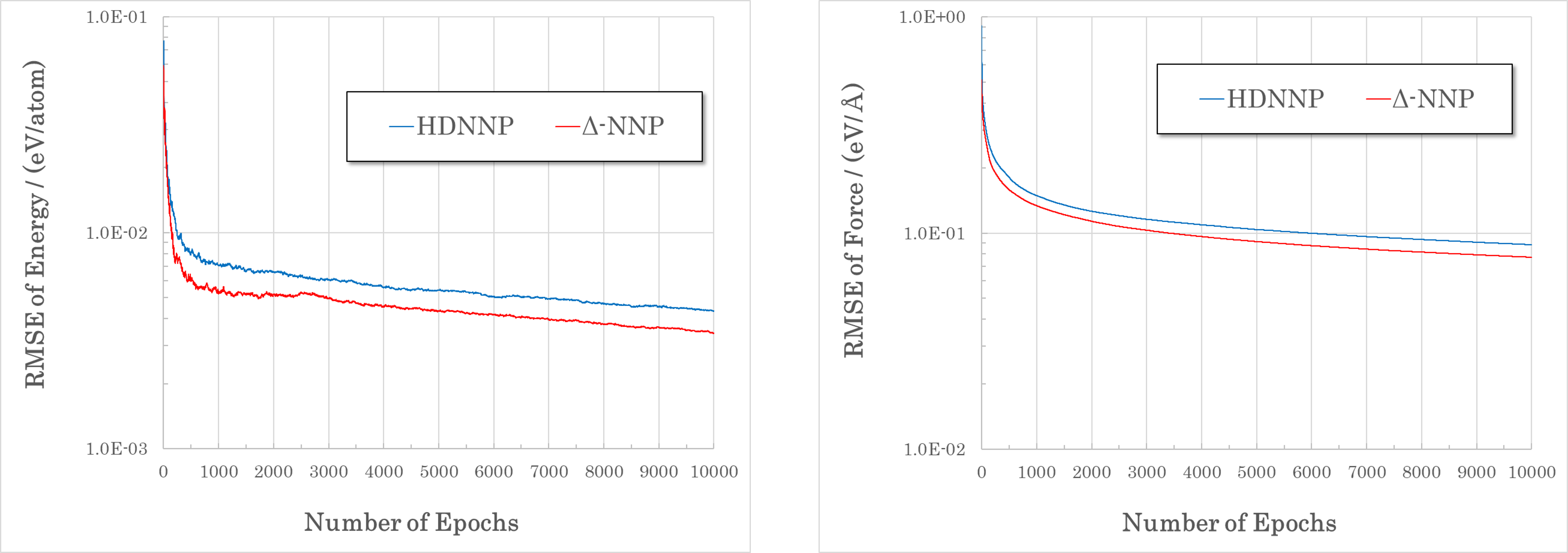
Figure: Δ-NNP and HDNNP were trained using the same training data (Li10GeP2S12, 6914 structures) and the RMSE was compared. Δ-NNP showed better convergence than HDNNP.
Δ-NNP using ReaxFF
In this method, ReaxFF[7]is used as the classical potential of Δ-NNP. ReaxFF is an many-body force field and can express energy/force better. In this product, only bond energy( ), Over-coordination energy(
 ), Under-coordination energy(
 ), Lone-pair energy(
 ) and van der Waals energy(
 ) are used as the ReaxFF energy. Existing ReaxFF parameters are used and no optimization is performed within this product. You can specify the contribution of ReaxFF by factor (mixing rate)
  , and the remaining is expressed by NNP.

Self-learning Hybrid Monte Carlo Method
The Self-learning hybrid Monte Carlo (SLHMC) method[6] is the method that can proceed simultaneous generation of training data and learning of neural network force fields. It is executed according to the following algorithm.
Advance some ab initio molecular dynamics calculations from the initial structure and use them as training data to create an initial neural network force field.
The structure is evolved in time by first-principles molecular dynamics calculations (NVE) using the neural network force field (
 ).
).Calculate the energy
 for the structure
  after time development by first-principles calculation.
Use the following transition probabilities
 to decide whether to adopt the structure by the Metropolis method.
If it is rejected, return the structure to
 and redefine the momentum
  with the Boltzmann distribution at temperature .
After repeating 1.~3. to some extent, retrain the neural network force field using the generated structures (only the adopted structures or all the structures including the rejected ones) as the training data.
Repeat 1.~3. and 4.
In this method, there is no need to even prepare the training data but only one initial structure, and then a neural network force field can be automatically created. A force field can always be created to the same standard because the time and effort required to create a force field can be greatly reduced, and that factors depending on the procedure such as the quality of training data are eliminated. Moreover, the time required for calculations can also be significantly reduced since it tends to be possible to reduce the number of training data.
Another feature of this method is that the ensemble of training data strictly matches the ensemble of the first-principles molecular dynamics calculations, since the transition probabilities (3.) of the Monte Carlo method are determined by first-principles calculations.
This product can also deform the cell by NPH before the time development of the structure (1.), or perform molecular dynamics calculation by NPH (not NVE) at the time development of the structure (1.). This will also include training data with different cell geometries, allowing this method to create force fields for materials with unknown lattice constants (densities). In this case, it is no longer a strict Monte Carlo method, but it can be used without problems for the purpose of creating a force field.